Antimicrobial therapy episodes

11 February 2024

Introduction

Hospital patients with suspected infection are often treated with empirical antibiotics. Antibiotic treatment is usually reviewed 24–72 hours later. This often results in changes to the choice of drug, its dose, and/or route of administration. Ideally, these decisions are informed by microbial culture results from biological samples such as blood or urine.

Understanding how antibiotics are used in the hospital underpins effective antimicrobial stewardship. This requires knowledge of the sequence of prescribing events and requires information on:

• the type of antibiotic (antibiotic class) used to initiate therapy
• subsequent changes to the original prescription, such as switching to a narrower/broader spectrum of antibiotic.

Ramses reconstructs prescribing events relating to an individual: it creates antimicrobial therapy episodes, which link the set of antimicrobial prescriptions administered consecutively or concurrently in a given patient.

Therapy episodes in Ramses

Motivating example

The diagrams below illustrates how to characterise prescribing events using Ramses.

A. Raw records B. Records linked into a therapy episode

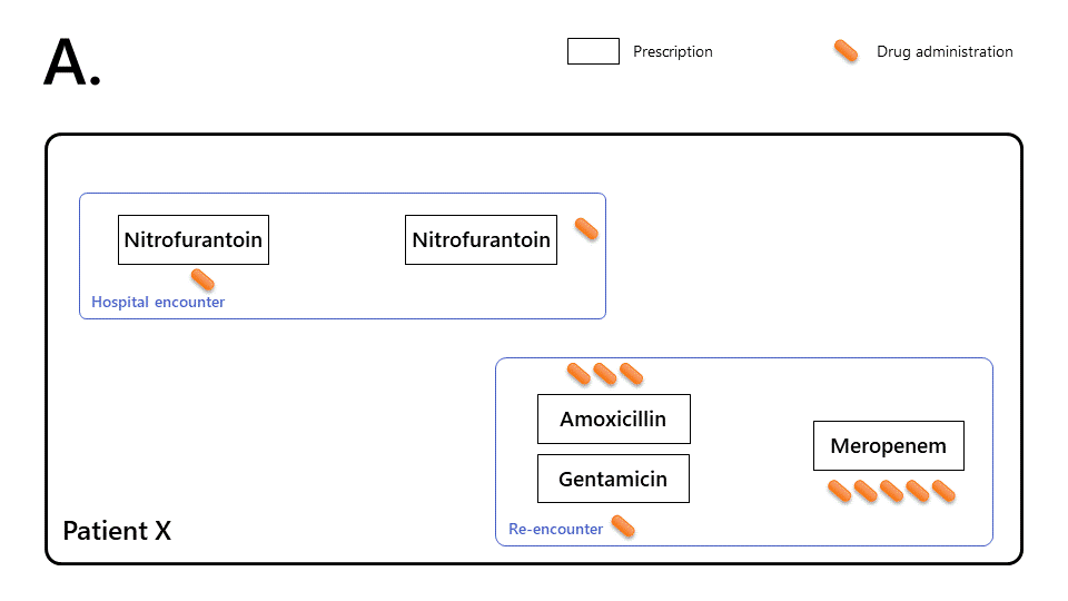
1. Based on unprocessed medical records alone, it is hard to characterise the chain of prescribing events.

   Patient X was prescribed nitrofurantoin (single dose + 3 day course) during a first encounter.

   Patient X re-presented to hospital 24 hours later and was treated with amoxicillin (1 day), gentamicin (single dose), and meropenem (5 day course).

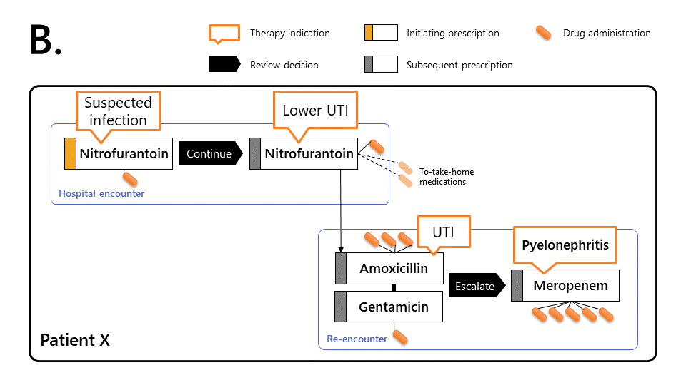
2. Ramses links prescriptions together (by transitive closure) to reconstruct the therapy episode, allowing more sophisticated observations:

   This makes it possible to determine that Patient X took antibiotics without interruption for 7 days.

   On first encounter, patient X was given a first dose of nitrofurantoin for a suspected lower urinary tract infection (UTI), then reviewed by a senior doctor and prescribed a three day course of the same antibiotic. The patient only spent one day in hospital during this period.

   During the following 24h, patient X’s worsening condition led them to re-present to hospital. Patient X was prescribed combination therapy (amoxicillin and a single dose of gentamicin). Patient X was prescribed combination therapy (amoxicillin and a single dose of gentamicin). The patient was reviewed 24 hours later, diagnosed with pyelonephritis and prescribed a 5-day course of meropenem.

Therapy episodes objects

Therapy episodes and therapy combinations are created automatically by Ramses when loading data (see methods). They are identified in the drug_prescriptions table in variables therapy_id and combination_id.

library(Ramses)
library(dplyr)
ramses_db <- create_mock_database("ramses-db.duckdb")

tbl(ramses_db, "drug_prescriptions") %>% 
  filter(patient_id == "99999999998") %>% 
  collect() %>% 
  select(patient_id, prescription_id, combination_id, 
         therapy_id, therapy_rank, prescription_text) %>% 
  glimpse()
#> Rows: 5
#> Columns: 6
#> $ patient_id        <chr> "99999999998", "99999999998", "99999999998", "999999…
#> $ prescription_id   <chr> "d7c0310a08cf9f0f318276125cd282ed", "7a0cb5555a43297…
#> $ combination_id    <chr> NA, NA, NA, "3e1c0e592a346d479aabc83513b4d812", "3e1…
#> $ therapy_id        <chr> "d7c0310a08cf9f0f318276125cd282ed", "d7c0310a08cf9f0…
#> $ therapy_rank      <dbl> 1, 2, 5, 3, 4
#> $ prescription_text <chr> "Nitrofurantoin ORAL 100mg 0 days", "Nitrofurantoin …

Therapy episodes are represented as objects of S4 class TherapyEpisode.

uti_episode <- TherapyEpisode(ramses_db, "d7c0310a08cf9f0f318276125cd282ed")
uti_episode
#> TherapyEpisode d7c0310a08cf9f0f318276125cd282ed 
#> Patient:   99999999998 
#> Start:     2015-03-01 20:00:00 UTC 
#> End:       2015-03-11 23:00:00 UTC 
#> 
#> Medications:
#>   > Nitrofurantoin ORAL 100mg 0 days
#>   > Nitrofurantoin ORAL 100mg 3 days
#>   > Amoxicillin ORAL 500mg 3 days
#>   > Gentamicin IV 350mg 0 days
#>   > Meropenem IV 1g 5 days
#> 
#> Database connection:
#> <duckdb_connection ae2f0 driver=<duckdb_driver f9d40 dbdir='ramses-db.duckdb' read_only=FALSE bigint=numeric>>

S4 class TherapyEpisode is capable of handling multiple therapy episodes at once.

TherapyEpisode(ramses_db, 
               c("d7c0310a08cf9f0f318276125cd282ed", 
                 "5528fc41106bb48eb4d48bc412e13e67"))
#> TherapyEpisode 5528fc41106bb48eb4d48bc412e13e67, d7c0310a08cf9f0f318276125cd282ed 
#> [total of 2 therapy episodes]
#> Patient(s):   99999999999, 99999999998 
#> 
#> Database connection:
#> <duckdb_connection ae2f0 driver=<duckdb_driver f9d40 dbdir='ramses-db.duckdb' read_only=FALSE bigint=numeric>>

For more information on S4 classes used in Ramses and their associated methods, see the Objects and classes vignette.

Longitudinal analysis

Therapy tables

Therapy episodes can be studied by creating a longitudinal, hour-by-hour matrix called ‘longitudinal table’.

longitudinal_table(uti_episode, collect = TRUE) %>% 
  select(t, therapy_start, therapy_end, t_start, t_end, parenteral)

This basic table can be enhanced with clinical features.

By default, route of therapy administration is indicated in the parenteral field:

• 1 indicates that all drugs are administered via parenteral route (eg intravenously)
• 0 indicates that at least one drug is administered via another route (eg orally)
• NA marks short gaps between prescriptions.

The parenteral_changes() function extracts transitions from intravenous to oral therapy. The example below shows just one prescribing sequence that included intravenous therapy. This sequence was initiated at \(t\) = 122, and ended at \(t\) = 242, without ever being converted to oral administration (NA).

parenteral_changes(uti_episode)
#> $d7c0310a08cf9f0f318276125cd282ed
#> $d7c0310a08cf9f0f318276125cd282ed[[1]]
#> [1] 122 242  NA

This function returns as many vectors as there are sequences of parenteral administration:

parenteral_changes(TherapyEpisode(ramses_db, "a028cf950c29ca73c01803b54642d513"))
#> $a028cf950c29ca73c01803b54642d513
#> $a028cf950c29ca73c01803b54642d513[[1]]
#> [1]   0 144  97
#> 
#> $a028cf950c29ca73c01803b54642d513[[2]]
#> [1] 146 316 219
#> 
#> $a028cf950c29ca73c01803b54642d513[[3]]
#> [1] 318 390  NA

In this example, parenteral therapy was first initiated at \(t\) = 0, then converted to oral administration at \(t\) = 97, until \(t\) = 144. A new sequence of parenteral therapy begins at \(t\) = 146, all within the same therapy episode.

Encounter tables

Encounters (hospitalisations) can also be used to generate longitudinal tables thanks to the Encounter() function. In the example below, an encounter table is created for the same patient 99999999998 for encounter 8895465895, which is the same admission during which antimicrobial therapy episode d7c0310a08cf9f0f318276125cd282ed was administered.

Like therapy tables, encounter tables can be enhanced with clinical features.

Encounter(ramses_db, "8895465895") %>% 
  longitudinal_table(collect = TRUE) %>% 
  select(t, admission_date, discharge_date, t_start, t_end)

Extended longitudinal tables

Both therapy and encounter tables can be extended so they begin earlier than the start of antimicrobial therapy, or the admission date, respectively. Doing so is controlled by the TherapyEpisode() and Encounter() functions to create the objects in the first place through an optional parameter extend_table_start. This parameter expresses how many hours earlier the table should start.

For example, the encounter table can be made to begin 5 hours before admission. This can be very useful if the patient is known to have stayed in the Emergency Department before being admitted:

Encounter(ramses_db, "8895465895", extend_table_start = 5) %>% 
  longitudinal_table(collect = TRUE) %>% 
  select(t, admission_date, discharge_date, t_start, t_end)

The extend_table_start parameter may also be used in the TherapyEpisode() function.

Adding clinical features

Several functions can enhance both therapy and encounter tables with variables characterising the clinical state and trajectory of the patient. For instance, we may be interested in temperature:

• clinical_feature_last() fetches the most recent temperature value.
• clinical_feature_mean() computes a running arithmetic mean of the temperature time series.
• clinical_feature_interval() computes the number of observations falling within and outside a specified interval (eg 36°C–38°C) or lying below/above a specified threshold (eg 38°C).
• clinical_feature_ols_trend() computes the Ordinary Least Square (OLS) trend; including the slope parameter, enabling to measure whether temperature has been rising/stable/falling.

The example below demonstrates how to classify a patient as hypothermic/afebrile/febrile:

example_sepsis <- TherapyEpisode(ramses_db, "4d611fc8886c23ab047ad5f74e5080d7") %>% 
  clinical_feature_last(observation_code = "8310-5", hours = 6) 

longitudinal_table(example_sepsis, collect = TRUE) %>% 
  mutate(
    febrile = case_when(
      last_temperature_6h < 36 ~ "hypothermic",
      between(last_temperature_6h, 36, 38) ~ "afebrile",
      last_temperature_6h > 38 ~ "febrile",
      TRUE ~ NA_character_
    )
  ) %>% 
  select(t, t_start, t_end, last_temperature_6h, febrile) %>% 
  filter(t < 50)
#> # A tibble: 50 × 5
#>        t t_start             t_end               last_temperature_6h febrile 
#>    <int> <dttm>              <dttm>                            <dbl> <chr>   
#>  1     0 2017-02-13 13:07:00 2017-02-13 14:07:00                36.9 afebrile
#>  2     1 2017-02-13 14:07:00 2017-02-13 15:07:00                36.9 afebrile
#>  3     2 2017-02-13 15:07:00 2017-02-13 16:07:00                36.8 afebrile
#>  4     3 2017-02-13 16:07:00 2017-02-13 17:07:00                36.8 afebrile
#>  5     4 2017-02-13 17:07:00 2017-02-13 18:07:00                36.8 afebrile
#>  6     5 2017-02-13 18:07:00 2017-02-13 19:07:00                36.9 afebrile
#>  7     6 2017-02-13 19:07:00 2017-02-13 20:07:00                36.8 afebrile
#>  8     7 2017-02-13 20:07:00 2017-02-13 21:07:00                36.8 afebrile
#>  9     8 2017-02-13 21:07:00 2017-02-13 22:07:00                36.1 afebrile
#> 10     9 2017-02-13 22:07:00 2017-02-13 23:07:00                36.1 afebrile
#> # ℹ 40 more rows

Another example below tracks the blood neutrophil count, which provides insights into the patient’s clinical progression following treatment. We want to know whether this parameter is going up, or down. The hours parameter is set to 48 hours: the function will look at all neutrophil counts in the last 48 hours. This should ensure we capture two recent values and can compute a slope.

clinical_feature_ols_trend(
  x = example_sepsis,
  observation_code = "751-8",
  hours = 48
) %>% longitudinal_table(collect = TRUE) %>% 
  select(t, t_start, ols_neutrophils_48h_slope, ols_neutrophils_48h_intercept, ols_neutrophils_48h_N) %>%
  filter(between(t, 10, 14) | between(t, 80, 84))
#> # A tibble: 10 × 5
#>        t t_start             ols_neutrophils_48h_slope ols_neutrophils_48h_int…¹
#>    <int> <dttm>                                  <dbl>                     <dbl>
#>  1    10 2017-02-13 23:07:00                    0.0867                     11.0 
#>  2    11 2017-02-14 00:07:00                    0.0867                     11.1 
#>  3    12 2017-02-14 01:07:00                    0.0867                     11.1 
#>  4    13 2017-02-14 02:07:00                    0.0867                     11.2 
#>  5    14 2017-02-14 03:07:00                    0.0867                     11.3 
#>  6    80 2017-02-16 21:07:00                   -0.0912                      6.01
#>  7    81 2017-02-16 22:07:00                   -0.0912                      5.92
#>  8    82 2017-02-16 23:07:00                   -0.0912                      5.82
#>  9    83 2017-02-17 00:07:00                   -0.0912                      5.73
#> 10    84 2017-02-17 01:07:00                   -0.0912                      5.64
#> # ℹ abbreviated name: ¹​ols_neutrophils_48h_intercept
#> # ℹ 1 more variable: ols_neutrophils_48h_N <dbl>

Note that the intercept is defined for \(t\) = t_start. In other words, its value corresponds to the linear (straight line) extrapolation of the trend to t_start.

We can see that, at the time of therapy initiation, the neutrophil count was increasing by an average 0.09 per nanoliter every hour (neutrophilia). After 80 hours (day 3), we find first evidence of the neutrophil count going down at a rate of 0.09 per nanoliter every hour, returning to a normal range (2–7.5 10⁹/L). Depending on the patient’s other vitals, this could indicate the infection is under control.

Methodology

Prescription linkage

Ramses links prescriptions together if:

• prescriptions share the same antiinfective_type: antibacterials are linked with antibacterials, antifungals with antifungals, etc.
• prescription_status is not "draft", "entered-in-error", "cancelled", or "unknown".

Ramses links prescriptions into episodes and combinations in two instances:

• by default, using the load_medications() function
• on request, by calling the create_therapy_episodes() function.

Both functions include a transitive_closure_controls argument, which controls parameters for linking prescriptions together into episodes and/or combinations, based on patterns of overlap or time elapsed between prescriptions (see defaults in the table below).

To change the default settings, consult the documentation ?transitive_closure_control.

Prescription overlap pattern classification rules and default settings (Dutey‐Magni et al. 2021)

Category	Pattern	Conditions for combination therapy	Conditions for continuation of therapy*
1		Ordered a max of 6h apart AND administrations separated by at the most 24h	Separated by at the most 36h
2		Ordered a max of 6h apart AND drug is identical AND first administrations separated by at the most 24h	Separated by at the most 36h
3		Never	Separated by at the most 36h
4		Never	Always
5		Ordered a max of 6h apart AND first administrations separated by at the most 24h	Always, unless combinations
6		Ordered a max of 6h apart AND first administrations separated by at the most 24h	Always, unless combinations
7		Never	Separated by at the most 36h

Notes:

• ○ denotes prescriptions for one-off administrations
• ▭ denotes regular prescriptions (including drugs to take home)
• \(*\) for continuation edges, only monotherapy prescriptions and the first prescriptions within combinations (by drug alphabetical order) are used
• in all categories, the date of first administration of (A) is anterior or equal to the date of first administration of (B).

References

Dutey‐Magni, P. F., M. J. Gill, D. McNulty, G. Sohal, A. C. Hayward, and L. Shallcross. 2021. “Feasibility study of hospital antimicrobial stewardship analytics using electronic health records.” JAC-Antimicrobial Resistance. https://doi.org/10.1093/jacamr/dlab018.