Ramses: R Package for Antimicrobial Stewardship & Surveillance
11 February 2024
Source:vignettes/Ramses.Rmd
Ramses.RmdIntroduction
Antimicrobial stewardship
Antimicrobial resistance jeopardizes many achievements of modern medicine, such as the ability to effectively treat infectious diseases or complete surgical procedures safely. Hospitals, alongside other inpatient facilities, make frequent use of categories of antibiotics which are most imminently eroding in effectiveness, the loss of which would have the most severe impact on health care systems (Sharland et al. 2018). They are thus at the forefront of the global effort to optimise the use of such antibiotics and sustain their effectiveness.
Ramses is an R package designed to support the
stewardship of antimicrobials in hospitals by facilitating the analysis
of routinely-collected electronic health records for:
Getting started
Setup
Ramses is currently in development. The latest stable
version can be installed using the devtools package.
devtools::install_github("ramses-antibiotics/ramses-package")Ramses comes with synthetic data for testing and
training purposes. You can use it to create a demonstration DuckDB
database fully loaded with synthetic electronic health records on a
local drive. No need for a database server.
Visualisation
You are now able to query the database and visualise admissions and episodes of antimicrobial therapy timeline below.
When hovered for a few seconds, timeline symbols display a tooltip containing detailed information.
therapy_timeline(Patient(conn = ramses_db,
                         id = "99999999999"),
                 date1 = as.Date("2017-02-01"),
date2 = as.Date("2017-03-01"))Data model
DBI::dbListTables(ramses_db)
#>  [1] "bridge_encounter_therapy_overlap"
#>  [2] "bridge_episode_prescription_initiation"
#>  [3] "bridge_episode_prescription_overlap"
#>  [4] "dbplyr_001"
#>  [5] "dbplyr_002"
#>  [6] "dbplyr_003"
#>  [7] "dbplyr_004"
#>  [8] "drug_administrations"
#>  [9] "drug_prescriptions"
#> [10] "drug_prescriptions_edges"
#> [11] "drug_therapy_episodes"
#> [12] "inpatient_diagnoses"
#> [13] "inpatient_episodes"
#> [14] "inpatient_investigations"
#> [15] "inpatient_ward_movements"
#> [16] "microbiology_isolates"
#> [17] "microbiology_specimens"
#> [18] "microbiology_susceptibilities"
#> [19] "patients"
#> [20] "ramses_tally"
#> [21] "ramses_tc_group"
#> [22] "reference_aware"
#> [23] "reference_icd"
#> [24] "reference_icd_ccs"
#> [25] "reference_icd_ccsr"
#> [26] "reference_icd_comorbidity"
#> [27] "reference_icd_infections"
Antibiotic consumption
Overview
Three main metrics are used to describe antimicrobial consumption in hospitals: Defined Daily Doses, Days on Therapy, and Length of Therapy. Definitions given by Stanić Benić et al. (2018) are reproduced below:
- Defined Daily Doses (DDDs) designate “the assumed average maintenance dose per day for a drug used for its main indication in adults” as defined by the WHO Collaborating Centre for Drug Statistics Methodology (WHO Collaborating Centre for Drug Statistics Methodology (2020)).
- Days of Therapy (DOTs) designate “the number of days that a patient receives antibiotics regardless of the dose. When a patient receives more than one antibiotic, more than one DOT may be counted”.
- Length of Therapy (LOT) designate “the number of days that a patient receives systemic antimicrobial agents, irrespective of the number of different antibiotics. Therefore, LOT will be lower than or equal to days of therapy (DOT) because the DOT is calculated for each antibiotic”.
Formulae are available from Ibrahim and Polk (2014) along with a discussion of rates which can be derived from these metrics (eg per 1,000 admissions, per 1,000 bed-days). Statistical adjustment of these metrics is discussed by Santen et al. (2018) and Yu et al. (2018).
The approach to create tables of antimicrobial consumption follows three steps:
- define the study population (encounters for which the above metrics should be derived)
- choose a bridge table to link encounters with prescriptions
- compute the metrics by aggregation.
DOTs/DDDs based on the episode of administration
Consumption can be attributed to specialty based on the specialty of
the episode during which the antibiotic is administered. In this case,
the appropriate bridge table is
bridge_episode_prescription_overlap.
study_pop <- tbl(ramses_db, "inpatient_episodes") %>%
  filter(main_specialty_code %in% c("100", "101", "300") &
           discharge_date >= "2016-01-01") %>%
  mutate(calendar_year = year(discharge_date),
         calendar_month = month(discharge_date))

consumption_num <- study_pop %>%
  left_join(tbl(ramses_db, "bridge_episode_prescription_overlap")) %>%
  group_by(calendar_year, calendar_month, main_specialty_code) %>%
  summarise(DOT_prescribed = sum(coalesce(DOT, 0.0)),
            DDD_prescribed = sum(coalesce(DDD_prescribed, 0.0)))
#> Joining with `by = join_by(patient_id, encounter_id, episode_number)`

consumption_denom <- study_pop %>%
  group_by(calendar_year, calendar_month, main_specialty_code) %>%
  summarise(bed_days = sum(ramses_bed_days))

consumption_rates <- full_join(consumption_denom, consumption_num) %>%
  collect() %>%
  mutate(month_starting = as.Date(paste0(calendar_year, "/", calendar_month, "/01")))
#> Joining with `by = join_by(calendar_year, calendar_month, main_specialty_code)`
#> Warning: Missing values are always removed in SQL aggregation functions.
#> Use `na.rm = TRUE` to silence this warning
#> This warning is displayed once every 8 hours.

head(consumption_rates)
#> # A tibble: 6 × 7
#> # Groups:   calendar_year, calendar_month [6]
#>   calendar_year calendar_month main_specialty_code bed_days DOT_prescribed
#>           <dbl>          <dbl> <chr>                  <dbl>          <dbl>
#> 1          2016              1 100                    16.7           10.9
#> 2          2017              7 100                    14.5           14.7
#> 3          2016              7 100                     8.73           4.89
#> 4          2017             11 100                    11.3            7.63
#> 5          2017             10 100                    27.1           14.4
#> 6          2016             11 100                     6.09           4.71
#> # ℹ 2 more variables: DDD_prescribed <dbl>, month_starting <date>
ggplot(consumption_rates,
       aes(x = month_starting,
           y = DOT_prescribed/bed_days*1000,
           group = main_specialty_code,
           color = main_specialty_code)) +
  geom_line() +
  scale_x_date(date_labels = "%b %Y") +
  xlab("Month") +
  ylab("Days of Therapy (DOTs)\nper 1,000 bed-days")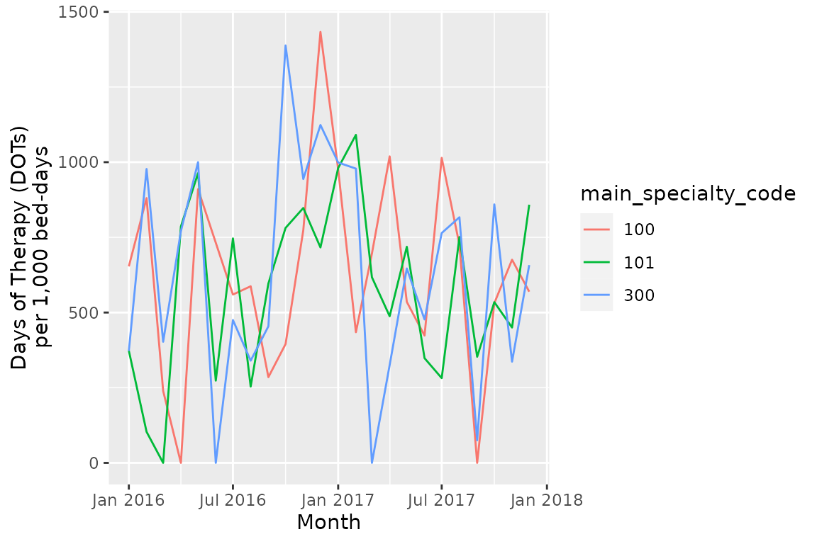
DOTs/DDDs based on the episode of initiation
Alternatively, consumption can be attributed to the episode when
prescriptions are issued (authoring_date field in
drug_prescriptions). In this case, the appropriate bridge
table is bridge_episode_prescription_initiation. This
amounts to attributing antibiotic consumption to the initial
prescriber.
consumption_num_init <- study_pop %>%
  left_join(tbl(ramses_db, "bridge_episode_prescription_initiation")) %>%
  group_by(calendar_year, calendar_month, main_specialty_code) %>%
  summarise(DOT_prescribed = sum(coalesce(DOT, 0.0)),
            DDD_prescribed = sum(coalesce(DDD_prescribed, 0.0)))
#> Joining with `by = join_by(patient_id, encounter_id, episode_number)`

consumption_denom_init <- study_pop %>%
  group_by(calendar_year, calendar_month, main_specialty_code) %>%
  summarise(
    bed_days = sum(ramses_bed_days),
    total_admissions = n_distinct(paste0(patient_id, encounter_id))
  )

consumption_rates_init <- full_join(consumption_denom_init, consumption_num_init) %>%
  collect() %>%
  mutate(month_starting = as.Date(paste0(calendar_year, "/", calendar_month, "/01")))
#> Joining with `by = join_by(calendar_year, calendar_month, main_specialty_code)`
ggplot(consumption_rates_init,
       aes(x = month_starting,
           y = DOT_prescribed/total_admissions*1000,
           group = main_specialty_code,
           color = main_specialty_code)) +
  geom_line() +
  scale_x_date(date_labels = "%b %Y") +
  xlab("Month") +
  ylab("Days of Therapy (DOTs)\nper 1,000 admissions")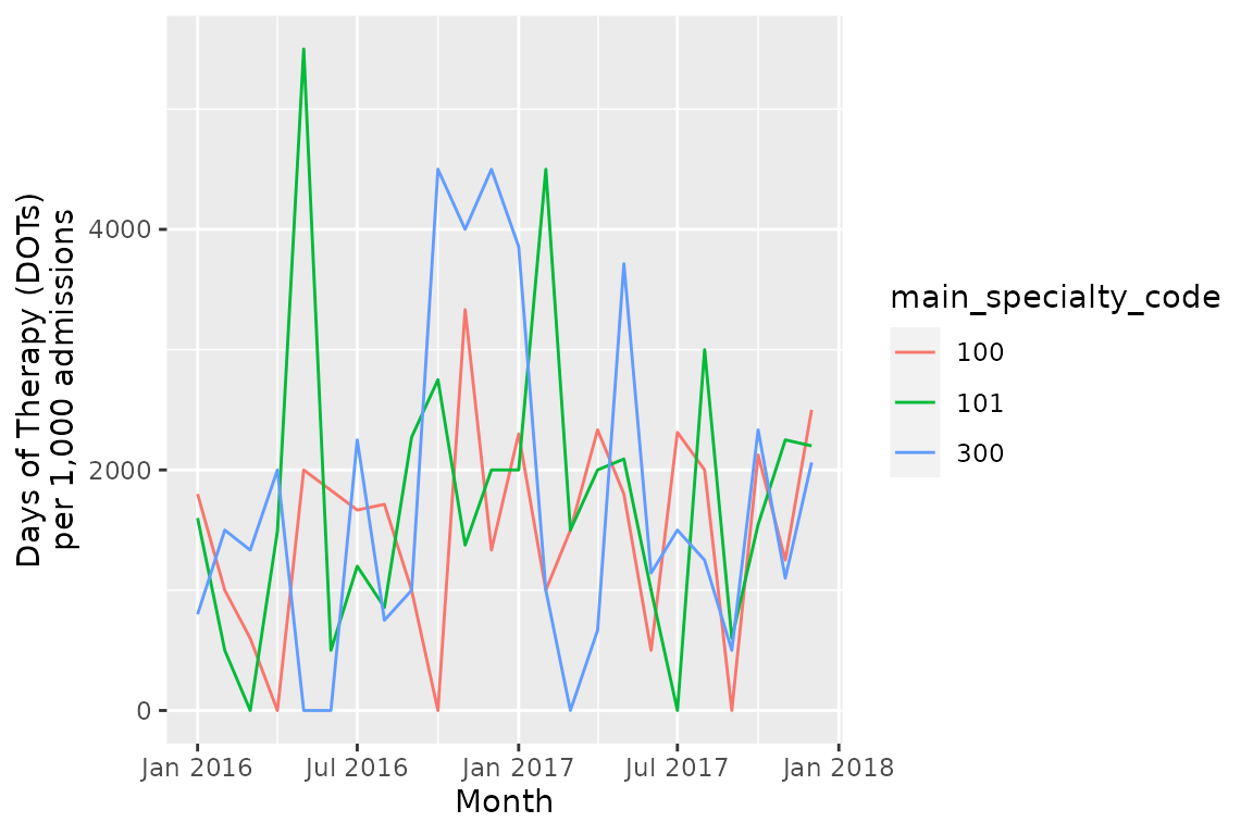
Length of therapy
Length of Therapy is the time elapsed during a prescribing episodes
(sequence of antimicrobial prescriptions separated by at the most 36
hours by default). To measure it, the bridge table
bridge_encounter_therapy_overlap is available. It calculate
the total LOT during between admission and discharge (excluding
to-take-home medications).
length_therapy_by_encounter <- study_pop %>%
  distinct(patient_id, encounter_id, admission_method) %>%
  left_join(tbl(ramses_db, "bridge_encounter_therapy_overlap")) %>%
  group_by(patient_id, encounter_id, admission_method) %>%
  summarise(LOT = sum(LOT, na.rm = T)) %>%
  collect()

length_therapy_by_encounter %>%
  group_by(admission_method) %>%
  summarise(
    `Total admissions` = n(),
    `Total admissions with therapy` = sum(!is.na(LOT)),
    `Mean LOT` = mean(LOT, na.rm = T),
    `Median LOT` = median(LOT, na.rm = T),
    percentile25 = quantile(x = LOT, probs = .25, na.rm = T),
    percentile75 = quantile(x = LOT, probs = .75, na.rm = T)
    ) %>%
  transmute(
    `Admission method` = case_when(
      admission_method == 1 ~ "Elective",
      admission_method == 2 ~ "Emergency"),
    `Total admissions`,
    `Mean LOT`,
    `Median LOT`,
    `Inter-quartile range` = paste0(
      formatC(percentile25, format = "f", digits = 1),
      "-",
      formatC(percentile75, format = "f", digits = 1)
    )
  ) %>%
knitr::kable(digits = 1)| Admission method | Total admissions | Mean LOT | Median LOT | Inter-quartile range |
|---|---|---|---|---|
| Elective | 46 | 4.3 | 3 | 0.9-5.3 |
| Emergency | 160 | 4.5 | 3 | 1.6-6.1 |
Consumption based on the type of antibiotic
To measure rates of prescribing by antibiotic class or AWaRe category, the query design is different because different dimensions are sought for the numerator and denominator.
Unlike before, this task takes three steps:
- compute numerator table
- compute denominator table
- join tables
consumption_aware_episodes_num <- tbl(ramses_db, "drug_prescriptions") %>%
  select(patient_id, prescription_id, ATC_code, ATC_route) %>%
  left_join(tbl(ramses_db, "reference_aware"),
            by = c("ATC_code", "ATC_route")) %>%
  select(patient_id, prescription_id, aware_category) %>%
  left_join(tbl(ramses_db, "bridge_episode_prescription_overlap")) %>%
  inner_join(study_pop) %>%
  group_by(calendar_year, calendar_month, aware_category) %>%
  summarise(DOT_prescribed = sum(coalesce(DOT, 0.0)))
#> Joining with `by = join_by(patient_id, prescription_id)`
#> Joining with `by = join_by(patient_id, encounter_id, episode_number)`

consumption_aware_episodes_denom <- study_pop %>%
  group_by(calendar_year, calendar_month) %>%
  summarise(bed_days =  sum(coalesce(ramses_bed_days, 0.0)))

consumption_aware_episodes <- left_join(
  consumption_aware_episodes_denom,
  consumption_aware_episodes_num
) %>%
  collect() %>%
  mutate(month_starting = as.Date(paste0(calendar_year, "/", calendar_month, "/01")),
         aware_category = factor(aware_category,
                                    levels = c("Access", "Watch", "Reserve")))
#> Joining with `by = join_by(calendar_year, calendar_month)`
aware_colours <- c(
  "Access" = "#1cb1d1",
  "Watch" = "#008ab1",
  "Reserve" = "#ff9667"
  )

ggplot(consumption_aware_episodes,
       aes(x = month_starting,
           y = DOT_prescribed/bed_days*1000,
           group = aware_category,
           color = aware_category)) +
  geom_line() +
  scale_x_date(date_labels = "%b %Y") +
  scale_color_manual(name = "AWaRe category",
                     values = aware_colours) +
  xlab("Month") +
  ylab("Days of Therapy (DOTs)\nper 1,000 bed-days")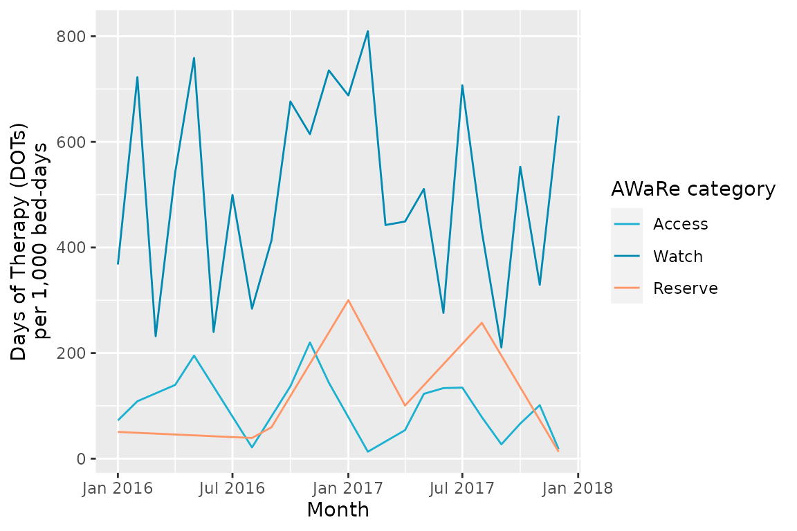
Once you are done
Always remember close database connections when you are finished.
DBI::dbDisconnect(ramses_db, shutdown = TRUE)